# install.packages(c("tidyverse", "survey", "labelled", "sjmisc", "naniar", "modelsummary"))

library(tidyverse)
library(survey)Exploring fear of crime in England: the role of area deprivation and crime victimisation
SC385 | L5. Introduction to survey methods | 2025/26
Introduction
Fear of crime usually refers to the fear of personally becoming a victim of particular types of crime, e.g., a question in a victim survey that asks respondents how likely they think it is that they will be burgled (or what have you) in the coming year. It is more common than victimization and is important because it can lead to stress and behavioral precautions that impinge on quality of life (Lane, 2015). To what extent area deprivation and crime victimisation explain fear of crime? There is an ongoing discussion about the role of neighbourhood characteristics on individual outcomes. Some studies have shown that deprived areas are more likely to tend to be racially segregated, have a higher crime rate, and low-quality public services in the US (e.g., Sampson et al., 1997).
The objective of this lab will be to explore how the level of fear of crime is related to area deprivation and crime victimisation in England. The analysis will also control for other individual characteristics, like personal income or education.
R packages and options
Before introducing the survey we will be using for the analysis, let’s load the packages and set the options for the analysis. If you do not have the packages installed, you can start by installing them using the code below.
The dataset
We will use the England and Wales Crime Survey (CSEW) 2017/18 teaching dataset for this lab. The CSEW is a large-scale, household-based survey designed to collect data on experiences of crime, perceptions of crime, and attitudes toward the criminal justice system. The survey is conducted throughout the year and collects data about the experiences of crime in the last 12 months. The interviews for the 2017/18 edition were conducted face-to-face, with sensitive topics addressed through a self-completion questionnaire. The survey is designed to be representative of the population living in private households in England and Wales.
The England and Wales Crime Survey (CSEW)
The CSEW aims to provide insights into crime trends over time, including those not reported to the police, and public perceptions of crime and safety.
The survey covers England and Wales and includes individuals aged 16 and over, with a separate module for children aged 10-15. All household members are invited to take part in the survey.
The survey uses a stratified, multi-stage random probability sample. A sample of postcode sectors (PSU) is selected from the postal address file. Then, addresses are selected within postcode sectors.
The 2017/18 CSEW interviewed approximately 35,000 adults and 3,000 children aged 10-15. The dataset you will use for the exercise is a subsample of the full dataset.
The data can be downloaded through the UK Data Service.
First, let’s read in the data you will find on Moodle in a RDS format. The dataset contains the responses of 32,101 adults to the individual interview and 22 variables. You can use the functions head() or glimpse() to have a first look at the dataset.
df <- read_rds("data/cse_2017-18_teaching.RDS")

head(df)| serial | worryx | wburgl | wmugged | wattack | wraceatt | carmot | cardamag | yrdeface | delibvio | imd_quint | income | sex | ageg | edu | bornuk | strata | psu | weight |
|---|---|---|---|---|---|---|---|---|---|---|---|---|---|---|---|---|---|---|
| 423023 | -0.2484040 | Fairly worried | Not very worried | Not very worried | Not at all worried | Yes | No | No | No | Q5 (Less deprived areas) | 15,000-29,999 | Male | 55-64 | Apprenticeship or A/AS level | Born in UK | 30011 | 11172802 | 0.6150459 |
| 423119 | -0.8156970 | Not very worried | Not at all worried | Not very worried | Not at all worried | No | NA | No | No | Q4 | Under 15,000 | Male | 16-24 | Apprenticeship or A/AS level | Born in UK | 30011 | 11172418 | 1.6044675 |
| 423211 | -0.5336742 | Not very worried | Not very worried | Not at all worried | Not very worried | Yes | No | No | No | Q2 | Under 15,000 | Male | 55-64 | None | Born in UK | 30011 | 11172294 | 1.1845964 |
| 423227 | 0.9187671 | Not very worried | Fairly worried | Fairly worried | Not very worried | Yes | No | No | No | Q3 | 15,000-29,999 | Female | 35-44 | Degree or diploma | Born in UK | 30011 | 11172730 | 0.5956991 |
| 423231 | -1.3814231 | Not at all worried | Not at all worried | Not at all worried | Not at all worried | Yes | No | No | No | Q4 | 15,000-29,999 | Male | 55-64 | None | Born in UK | 30011 | 11172918 | 1.7307217 |
| 423323 | -0.8141301 | Not very worried | Not very worried | Not at all worried | Not at all worried | Yes | No | No | No | Q5 (Less deprived areas) | 30,000-49,999 | Male | 35-44 | Degree or diploma | Born in UK | 30011 | 11172970 | 1.3163648 |
Exploring the dataset
The function var_label of the package labelled can extract the label of each variable in the data frame. The code below is a simple way to generate a data frame with two columns: the variable name and the label.
labelled::var_label(df) %>%
  as_tibble() %>% # transform the output of var_label into a tibble object
pivot_longer(everything(), names_to = "variable_name", values_to = "variable_label") # reshape the data frame from a wide format to long format (more convenient for exploring the data)| variable_name | variable_label |
|---|---|
| serial | Serial number (6 digits) |
| worryx | Worry about being a victim of crime (high score = high level of worry) |
| wburgl | How worried about having your home broken into |
| wmugged | How worried about being mugged and robbed |
| wattack | How worried about being physically attacked by strangers |
| wraceatt | How worried about being attacked because of skin colour, ethnic origin or religi |
| carmot | If has a car ot motorcycle |
| cardamag | If vehicle tampered with or damaged |
| yrdeface | If anything was damaged outside current residence |
| delibvio | If anyone has deliberately used force/violence on adult respondent |
| imd_quint | English Index of Multiple Deprivation 2015 (quintiles) |
| income | What is your personal (and partners) gross income |
| sex | Adult number 1 (respondent): Sex |
| ageg | Age group (7 bands) |
| edu | Respondent education (5 categories) |
| bornuk | Person was born in the UK |
| strata | Stratum (2015 definition) |
| psu | PSU (2015 definition) |
| weight | Individual level weight (mean=1) |
Analysis objective
The objective of this lab is to analyse whether the level of fear of crime is related to area deprivation and crime victimisation controlling for other demographic factors: sex, age, education, personal income, and whether the person was born in the UK.
To measure fear of crime we will use the variable
worryx. Higher scores in the variable indicate a higher level of worry about suffering a crime. This variable is derived from five items in the survey that measure how worried was that person about:having their home broken into (
wburgl)being mugged and robbed (
wmugged)being physically attacked by strangers (
wattack)being attacked because of skin colour, ethnic origin or religion (
wraceatt)
The analysis will use the variable
worryx.To measure crime victimisation we will use three variables that identify whether the respondent has been a victim of at least one type of crime in the last 12 months:
If vehicle tampered with or damaged (
cardamag)If anything was damaged outside current residence (
yrdeface)If anyone has deliberately used force/violence on adult respondent (
delibvio)
To measure the deprivation of the area where the respondent lives, we will use the variable Index of multiple Deprivation (IMD), which is an index that ranks the neighbourhoods in England from the most deprived to the least deprived. The IMD is a composite measure that includes income, employment, health, education, crime, and living environment.
Index of Multiple Deprivation (IMD)
The Index of Multiple Deprivation (IMD) measures relative deprivation in small areas across each of the countries of the United Kingdom.
Areas are ranked from the most deprived area (rank 1) to the least deprived area.
Each country measures deprivation in a slightly different way but the broad themes include income, employment, education, health, crime, barriers to housing and services, and the living environment.
The statistical unit areas used to provide indices of relative deprivation across the country are Lower layer Super Output Areas (LSOAs) [England, Wales], Data Zones [Scotland] and Super Output Areas or Wards [Northern Ireland].
More information about the IMD.
The analysis will be conducted in two steps:
Preparing variables for the analysis: dealing with missing values. We will explore the data and identify the missing values in the variables and will make decisions about how to deal with the missing values in these variables.
Exploring the factors related to fear of crime. We will estimate the relationship between the level of fear of crime, area deprivation and crime victimisation using a linear regression model. This will be an opportunity to learn how to estimate the model using the
surveypackage in R, which takes into account some information about the complex sample design and weights to adjust for non-response.
1. Preparing the variables for the analysis: dealing with missing values
Types of missing data
Planned missingness. The researcher plans that some questions are not going to be presented to some respondents:
A long questionnaire might be split into a common set of questions that are asked to all respondents and a different set of questions that are asked to a random subset.
Some questions might be asked only to those who meet certain criteria. For example, questions about the experience of using public transport might be asked only to those who use public transport.
Unplanned missingness. Sometimes a respondent refuses to answer a question or, in self-administered mode, skips the questions. This can also happen by mistake. The result is that we do not have information about this question for this respondent.
Non-substantive responses. There are some responses that might be taken as substantive or missing depending on the research question and the objectives of the analysis. For example, a don’t know category is relevant if you intend to measure knowledge.
For a comprehensive guide on missing data in surveys read (Reid and Allum, 2019).
Exercise 1. Identifying and dealing with missing values
The first step in the analysis is to explore the data and identify the missing values. Before starting with the analysis, the analyst should have a clear answer to the following questions: What type and how many missing values are in the data? How can they affect the analysis? Which decisions, if any, do I need to make before proceeding with the analysis? This exercise will guide you through the process of identifying the missing values in the dataset.
E1.1 | What is the proportion of missing values in the dependent and independent variables?
Produce descriptives to examine the variables that will be included in the analysis: worryx, sex, ageg, edu, income, bornuk, cardamag , yrdeface, delibvio and imd_quint.
What proportion of missing values do you observe for each variable? Which variables would need some preparation before fitting the linear regression model?
a) Produce frequency tables of the categorical and ordinal variables (all except worryx). You can use the function select to select these variables and then use the function sjmisc::frq() to produce the frequency tables. The frequency tables will allow us to explore the variables and identify possible missing values. What proportion of missing values do you observe for each variable?
Selecting multiple variables: selector helpers
R has some helper functions to select multiple variables at once. The colon operator : can be used to select a range of variables. For example, var1:var3 will select all variables from var1 to var3. The c() function can be used to select multiple variables. For example, c(var1, var2, var3) will select the variables var1, var2, and var3.
If you use tidyverse (i.e., dplyr package) for data management some additional helpers are available:
starts_with("prefix")selects all variables that start with “prefix”.ends_with("suffix")selects all variables that end with “suffix”.contains("pattern")selects all variables that contain “pattern”.everything()selects all variables.
More information (and helper functions) are available at tidy select.
💡 Solution E1.1 a)
As you can see below, some variables such as sex, ageg and imd_quint have no missing values. Other variables have a small number (<1%) of user missing values (i.e., NA, “Refused” or “Don’t Know”).
However, the variables cardamag has a high number of system missing (<NA>). Later in the exercise we will determine what is causing these missing values.
The variable income has also a higher number of missing values. Some people did not know or refused to answer the question. The variable income is a key variable in our analysis, so we need to decide how to deal with the missing values in this variable.
The frequency tables are also useful to identify the levels (or categories) that need to be set as missing for the analysis. For example, the variables cardamag, yrdeface, delibvio and bornuk have a category “Refused” and “Don’t know” that should be set as missing NA.
df %>% select(cardamag:bornuk) %>% sjmisc::frq() If vehicle tampered with or damaged (cardamag) <categorical>
# total N=7916 valid N=6350 mean=1.95 sd=0.23
Value | N | Raw % | Valid % | Cum. %
--------------------------------------------
Yes | 318 | 4.02 | 5.01 | 5.01
No | 6023 | 76.09 | 94.85 | 99.86
Refused | 1 | 0.01 | 0.02 | 99.87
Don't know | 8 | 0.10 | 0.13 | 100.00
<NA> | 1566 | 19.78 | <NA> | <NA>
If anything was damaged outside current residence (yrdeface) <categorical>
# total N=7916 valid N=7916 mean=1.99 sd=0.13
Value | N | Raw % | Valid % | Cum. %
--------------------------------------------
Yes | 115 | 1.45 | 1.45 | 1.45
No | 7794 | 98.46 | 98.46 | 99.91
Refused | 2 | 0.03 | 0.03 | 99.94
Don't know | 5 | 0.06 | 0.06 | 100.00
<NA> | 0 | 0.00 | <NA> | <NA>
If anyone has deliberately used force/violence on adult respondent (delibvio) <categorical>
# total N=7916 valid N=7916 mean=1.99 sd=0.12
Value | N | Raw % | Valid % | Cum. %
--------------------------------------------
Yes | 110 | 1.39 | 1.39 | 1.39
No | 7802 | 98.56 | 98.56 | 99.95
Refused | 2 | 0.03 | 0.03 | 99.97
Don't know | 2 | 0.03 | 0.03 | 100.00
<NA> | 0 | 0.00 | <NA> | <NA>
English Index of Multiple Deprivation 2015 (quintiles) (imd_quint) <categorical>
# total N=7916 valid N=7916 mean=3.03 sd=1.40
Value | N | Raw % | Valid % | Cum. %
----------------------------------------------------------
Q1 (Most deprived areas) | 1509 | 19.06 | 19.06 | 19.06
Q2 | 1548 | 19.56 | 19.56 | 38.62
Q3 | 1632 | 20.62 | 20.62 | 59.23
Q4 | 1626 | 20.54 | 20.54 | 79.78
Q5 (Less deprived areas) | 1601 | 20.22 | 20.22 | 100.00
<NA> | 0 | 0.00 | <NA> | <NA>
What is your personal (and partners) gross income (income) <categorical>
# total N=7916 valid N=7916 mean=2.77 sd=1.44
Value | N | Raw % | Valid % | Cum. %
------------------------------------------------
Under 15,000 | 1860 | 23.50 | 23.50 | 23.50
15,000-29,999 | 1998 | 25.24 | 25.24 | 48.74
30,000-49,999 | 1604 | 20.26 | 20.26 | 69.00
50,000 or over | 1453 | 18.36 | 18.36 | 87.35
Refused | 590 | 7.45 | 7.45 | 94.81
Don't Know | 411 | 5.19 | 5.19 | 100.00
<NA> | 0 | 0.00 | <NA> | <NA>
Adult number 1 (respondent): Sex (sex) <categorical>
# total N=7916 valid N=7916 mean=1.53 sd=0.50
Value | N | Raw % | Valid % | Cum. %
----------------------------------------
Male | 3691 | 46.63 | 46.63 | 46.63
Female | 4225 | 53.37 | 53.37 | 100.00
<NA> | 0 | 0.00 | <NA> | <NA>
Age group (7 bands) (ageg) <categorical>
# total N=7916 valid N=7916 mean=4.19 sd=1.81
Value | N | Raw % | Valid % | Cum. %
---------------------------------------
16-24 | 529 | 6.68 | 6.68 | 6.68
25-34 | 1187 | 14.99 | 14.99 | 21.68
35-44 | 1312 | 16.57 | 16.57 | 38.25
45-54 | 1359 | 17.17 | 17.17 | 55.42
55-64 | 1266 | 15.99 | 15.99 | 71.41
65-74 | 1252 | 15.82 | 15.82 | 87.23
75+ | 1011 | 12.77 | 12.77 | 100.00
<NA> | 0 | 0.00 | <NA> | <NA>
Respondent education (5 categories) (edu) <categorical>
# total N=7916 valid N=7880 mean=2.93 sd=1.24
Value | N | Raw % | Valid % | Cum. %
--------------------------------------------------------------
None | 1563 | 19.74 | 19.84 | 19.84
O level/GCSE | 1353 | 17.09 | 17.17 | 37.01
Apprenticeship or A/AS level | 1381 | 17.45 | 17.53 | 54.53
Degree or diploma | 3242 | 40.96 | 41.14 | 95.67
Other | 341 | 4.31 | 4.33 | 100.00
<NA> | 36 | 0.45 | <NA> | <NA>
Person was born in the UK (bornuk) <categorical>
# total N=7916 valid N=7916 mean=1.84 sd=0.37
Value | N | Raw % | Valid % | Cum. %
---------------------------------------------
Born abroad | 1264 | 15.97 | 15.97 | 15.97
Born in UK | 6640 | 83.88 | 83.88 | 99.85
Refused | 11 | 0.14 | 0.14 | 99.99
Don't Know | 1 | 0.01 | 0.01 | 100.00
<NA> | 0 | 0.00 | <NA> | <NA>b) Produce descritive table of the continuous variable worryx (dependent variable). You can use the functions sjmisc::descr() or summary() to obtain basic descriptives and the number (or percentage) of missing values. What proportion of missing values do you observe for worryx?
Note that higher values of worryx indicate a higher level of worry about suffering a crime, while lower values indicate a lower level of worry.
💡 Solution E1.1 b)
As you can see below, only 174 cases (2.2%) of all observations are missing for the variable worryx.
summary(df$worryx) Min. 1st Qu. Median Mean 3rd Qu. Max. NA's
-1.38142 -0.77283 -0.22938 -0.01316 0.36176 2.88169 174 E1.2 | Why the variable (cardamg) has a ~20% missing values (<NA>)?
a) The variable cardamag is about the respondents’ cars or motorcycles. It is time to look at the data frame (or questionnaire) to see whether these variables are planned or unplanned missingness. Identify the variable that measures whether the respondent has a car or motorcycle and produce cross-tabs using the function table(). Are the <NA> of these variables planned or unplanned missingness? How would you treat these missing values in the analysis?
💡 Solution E1.2 a)
The cross-tabs below show that the variable cardamag is only asked to those who own a car or motorcycle. Note that those who do not have a car or motorcycle carmot == "No" or refused to answer the question are missing at cardamag. For the purpose of our analysis, we can ignore the missing values in these variables (<NA>) and recode the <NA> as "No" at cardamag.
table(df$carmot, df$cardamag, useNA = "always")
           Yes   No Refused Don't know <NA>
  Yes      318 6023       1          8    0
  No         0    0       0          0 1565
  Refused    0    0       0          0    1
  <NA>       0    0       0          0    0
b) Recode the variable cardamag so that the <NA> values are recoded to "No". An issue to produce this recode is how to specify that the cases with <NA> are missing values. The function fct_na_value_to_level can be used to set the missing values as a level of the factor. See the example below to learn how it works.
Dealing with factors in R: the
forcats package
The forcats package provides a set of functions to work with factors in R.
fct_recode()can be used to recode the levels of a factor.fct_collapse()can be used to collapse the levels of a factor into new levels.
Sometimes we need to manipulate NA values as a level of the factor. The function fct_na_value_to_level() can be used to set the missing values as a level of the factor (see example below).
The forcats package is part of tidyverse and all its functions start with fct_. The forcats functions used to transform variables can be called within mutate(). More information are available at forcats.
# EXAMPLE: recode the variable education (edu) to a factor with three levels:
# "Degree", "No degree" and "Missing". The misisng category should include those
# with NA and those responding "Other" to the education question. This is easier
# to do with fct_collapse() function.

# 1. Set the missing values as a level of the factor
table(df$edu, useNA = "always")
                        None                 O level/GCSE
                        1563                         1353
Apprenticeship or A/AS level            Degree or diploma
                        1381                         3242
                       Other                         <NA>
341 36 levels(df$edu) # the NA is not a level of the factor[1] "None" "O level/GCSE"
[3] "Apprenticeship or A/AS level" "Degree or diploma"
[5] "Other" # we need to set NA as a level of the factor to manipulate it.
# The function fct_na_value_to_level() can do this.
df <- df %>%
mutate(edu = fct_na_value_to_level(edu)) # set the missing values as a level
# check that now NA is a level so we can manipulate it.
levels(df$edu)[1] "None" "O level/GCSE"
[3] "Apprenticeship or A/AS level" "Degree or diploma"
[5] "Other" NA # 2. Use fct_collapse() to recode the variable.
df <- df %>%
mutate(edu3 = fct_collapse(edu,
Degree = "Degree or diploma",
Missing = c(NA, "Other"),
other_level = "No degree"
))
table(df$edu, df$edu3, useNA = "always")
                               Degree Missing No degree <NA>
  None                              0       0      1563    0
  O level/GCSE                      0       0      1353    0
  Apprenticeship or A/AS level      0       0      1381    0
  Degree or diploma              3242       0         0    0
  Other                             0     341         0    0
  <NA>                              0      36         0    0
💡 Solution E1.2 b)
 df <- df %>%
    mutate(cardamag = fct_na_value_to_level(cardamag), ## set the missing values NA as a level so we can recode it
           cardamag = fct_collapse(cardamag,
                                   No = c("No", NA)))

## check the variable
table(df$cardamag, useNA = "always")
       Yes         No    Refused Don't know       <NA>
       318       7589          1          8          0
E1.3 | Focusing on the variable personal income (income), what are the sociodemographic characteristics of the sample members who did not provide a substantive answer to this question compare to those who didn’t?
a) Generate the variable income_miss that takes “Missing” if the income variable is <NA>, Refused or Don't know and “Non-missing” otherwise. Use the function mutate and fct_collapse to create the new variable. You can use the function fct_na_level_to_value() from the package forcats to set the missing values as a level of the factor.
💡 Solution E1.3 a)
 df <- df %>%
    mutate(income = fct_na_value_to_level(income), ## set the missing values NA as a level
            income_miss = fct_collapse(income,
                                        Missing = c("Refused",
                                                  "Don't Know",
                                                  NA),
                                      other_level = "Non-missing"))

## check the variable
table(df$income, df$income_miss, useNA = "always")
                 Missing Non-missing <NA>
  Under 15,000         0        1860    0
  15,000-29,999        0        1998    0
  30,000-49,999        0        1604    0
  50,000 or over       0        1453    0
  Refused            590           0    0
  Don't Know         411           0    0
  <NA>                 0           0    0
b) Produce a cross-tab of the new variable income_miss with the variables sex, ageg, edu, bornuk and imd_quint. What are the sociodemographic characteristics of the sample members who did not provide a substantive answer to the question about their personal income? Could these differences affect the results of the analysis (e.g., regression coefficients)? You can use the sjmisc::flat_table() function to produce the cross-tab with row or column percentages.
Using
sjmisc::flat_table() to produce cross-tabs
The function sjmisc::flat_table() can be used to produce cross-tabs. The function has several arguments to control the output of the table. The argument margin can be used to produce row or column percentages. The argument show_na can be used to show the missing values in the table. The argument show_total can be used to show the total of the table. This function is an alternative to table() and prop.table() functions in base R.
More information about sjmisc.
# EXAMPLE: Use flat_table() to produce a cross-tab of two variables
# from the data frame df.
# margin can be 'counts', 'row', 'col' or 'cell'.

sjmisc::flat_table(df, edu, sex, margin = "col")
sex Male Female
edu
None 18.28 21.19
O level/GCSE 14.66 19.36
Apprenticeship or A/AS level 21.41 14.13
Degree or diploma 40.94 41.32
Other 4.71 4.00💡 Solution E1.3 b)
People who are older, have a lower level of education and were born abroad are less likely to report their income. The variable income_miss is not missing at random.
sjmisc::flat_table(df, sex, income_miss, margin = "row") income_miss Missing Non-missing
sex
Male 11.35 88.65
Female 13.78 86.22sjmisc::flat_table(df, ageg, income_miss, margin = "row") income_miss Missing Non-missing
ageg
16-24 15.88 84.12
25-34 9.27 90.73
35-44 10.14 89.86
45-54 10.60 89.40
55-64 13.19 86.81
65-74 13.34 86.66
75+ 19.39 80.61sjmisc::flat_table(df, edu, income_miss, margin = "row") income_miss Missing Non-missing
edu
None 19.32 80.68
O level/GCSE 11.46 88.54
Apprenticeship or A/AS level 10.79 89.21
Degree or diploma 9.78 90.22
Other 14.66 85.34sjmisc::flat_table(df, bornuk, income_miss, margin = "row") income_miss Missing Non-missing
bornuk
Born abroad 16.77 83.23
Born in UK 11.73 88.27
Refused 90.91 9.09
Don't Know 0.00 100.00c) Produce a box plot of the variable worryx by income_miss. Do those who did not provide information about their income have different levels of worry about suffering a crime? Could these differences affect the results of the analysis (e.g., regression coefficients)? You can use ggplot2 function to produce the boxplot (see example below).
Using
ggplot2 to produce boxplots
The ggplot2 package provides a set of functions to produce data visualisations in R. It is based on the Grammar of Graphics (Wilkinson, 2005). The basic idea is to build a plot layer by layer. The first layer is the data, the second layer is the aesthetic mapping, and the third layer is the geometric object.
- The function
ggplot(data, mapping)is used to create a ggplot object. - The function
geom_boxplot()tells ggplot2 that you want the information displayed with a boxplot. - The functions are combined using the
+operator.
ggplot2 package information is available at ggplot2.
How to interpret a boxplot?
- Center: The median line inside the box shows the center of the data.
- Spread: The length of the box shows the interquartile range (IQR), which is the spread of the middle 50% of the data. The total length of the plot (max - min) shows the overall range.
- Skewness: The position of the median within the box and the relative lengths of the whiskers can indicate the symmetry or skew of the data.
- Outliers: Any data points that fall outside the whiskers are often shown as individual points, indicating potential outliers.
# EXAMPLE: boxplot of worryx by edu.

ggplot(df, aes(x = edu, y = worryx)) +
  geom_boxplot()
Warning: Removed 174 rows containing non-finite outside the scale range
(`stat_boxplot()`).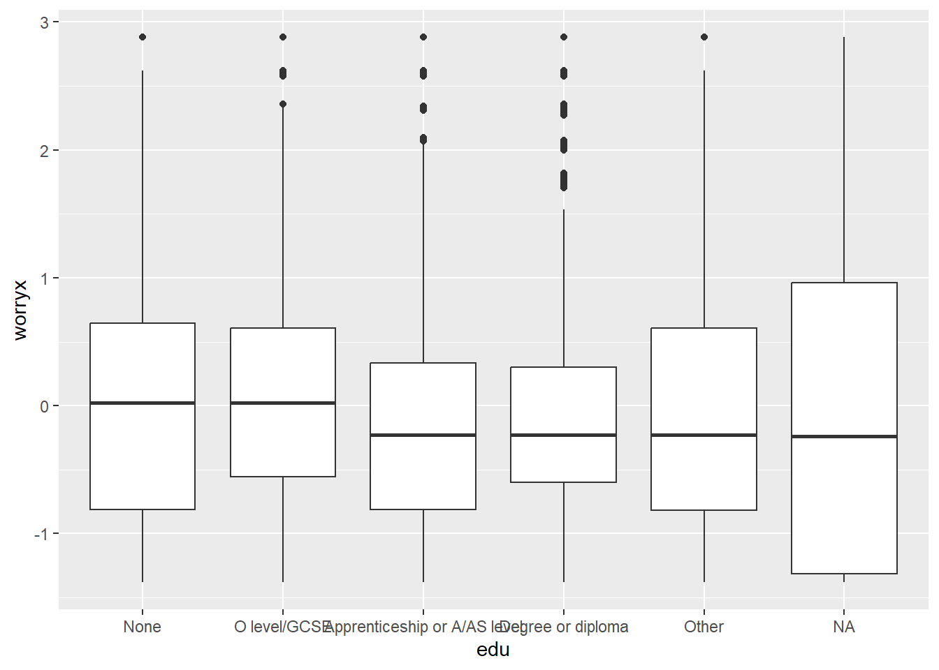
💡 Solution E1.3 c)
Those not providing information about their income show a similar distribution of the variable worryx compared to those who provided information.
ggplot(df, aes(x = income_miss, y = worryx)) +
  geom_boxplot()
Warning: Removed 174 rows containing non-finite outside the scale range
(`stat_boxplot()`).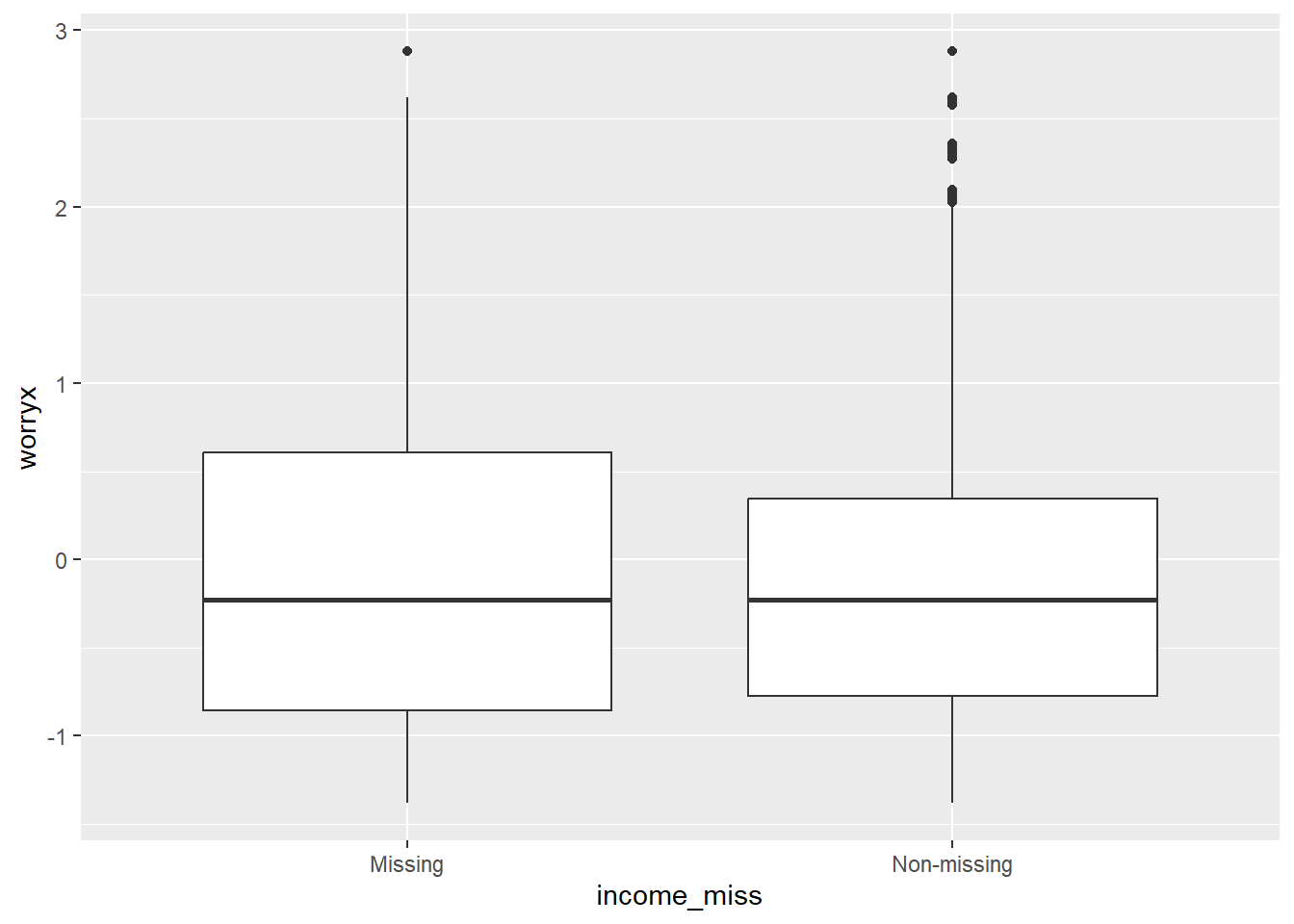
E1.4 | How to deal with missing values? Alternatives available for the analyst
Dealing with missing values in survey data analysis
Listwise deletion or complete case analysis. The analyst can decide to exclude all cases with missing values in any of the variables involved in the analysis. For example, if you are producing cross-tabs using sex, age and income, all cases that have a missing values for any of the three variables will be excluded from the analysis.
Pairwise deletion. The analyst can decide to exclude cases with missing values only in the variables involved in the analysis. For example, in the scenario mentioned above, only the cases with missing values at sex or age would be excluded from the sex~age cross-tab, whilst only the cases with missing values at age or income would be excluded from the crosstab age~income. As a result each of the cross-tabs will involve a different number of cases.
This approach can lead to biased estimates if the missing values are not missing completely at random (MCAR), i.e. if those excluded due to missingness are different from those used in the analysis.
- Imputation. There is a third, more complex set of alternatives that involve statistical methods to estimate the likely response of the respondents who did not provide a valid answer. This is called imputation. There are several methods to impute missing values, such as mean imputation, regression imputation, multiple imputation, etc. You can learn more about them in (van Buuren, 2018).
Since our objective is to estimate a regression model we will use a complete case analysis (listwise deletion). This means that we will exclude all cases with missing values in any of the variables involved in the analysis: worryx, sex, ageg, edu, bornuk, income, cardamag, yrdeface, delibvio and imd_quint will be used in the analysis.
a) We need to set as missing values <NA> the levels of some variables that have “Refused” or “Don’t know”. The function fct_na_level_to_value() can be used to set the missing values as a level of the factor.
Setting values as missing
<NA> in R
There are some alternatives to set values as missing in R:
You can use R base to identify the cases that you want to set as missing and then use the assignment operator
<-to set the value as missing. For example,df$income[df$income == "Refused"] <- NAwill set the value “Refused” as missing in the variableincome.The function
na_if()can be used to set a value as missing. For example,na_if(df$income, "Refused")will set the value “Refused” as missing in the variablex. The functionna_if()can be used withinmutate().The
forcatspackage provides the functionfct_na_level_to_value()to set one or more levels of a factor as missing values. For example,fct_na_level_to_value(df$income, "Refused")will set the value “Refused” as missing in the variableincome. The function can be used withinmutate().
💡 Solution E1.4 a)
In the next chunk of code we set the missing values in the variables income, cardamag, yrdeface, bornuk and delibvio as <NA>.
## Set factor levels as NA for income and bornuk
df <- df %>%
  mutate(income = fct_na_level_to_value(income, c("Refused", "Don't Know")),
         cardamag = fct_na_level_to_value(cardamag, c("Refused", "Don't know")),
         yrdeface = fct_na_level_to_value(yrdeface, c("Refused", "Don't know")),
         delibvio = fct_na_level_to_value(delibvio, c("Refused", "Don't know")),
         bornuk = fct_na_level_to_value(bornuk, c("Refused", "Don't Know"))
         )

## check that the non-valid levels are set as NA
df %>%
  select(income, cardamag, yrdeface, delibvio, bornuk) %>%
  sjmisc::frq()
What is your personal (and partners) gross income (income) <categorical>
# total N=7916 valid N=6915 mean=2.38 sd=1.09
Value | N | Raw % | Valid % | Cum. %
------------------------------------------------
Under 15,000 | 1860 | 23.50 | 26.90 | 26.90
15,000-29,999 | 1998 | 25.24 | 28.89 | 55.79
30,000-49,999 | 1604 | 20.26 | 23.20 | 78.99
50,000 or over | 1453 | 18.36 | 21.01 | 100.00
<NA> | 1001 | 12.65 | <NA> | <NA>
If vehicle tampered with or damaged (cardamag) <categorical>
# total N=7916 valid N=7907 mean=1.96 sd=0.20
Value | N | Raw % | Valid % | Cum. %
---------------------------------------
Yes | 318 | 4.02 | 4.02 | 4.02
No | 7589 | 95.87 | 95.98 | 100.00
<NA> | 9 | 0.11 | <NA> | <NA>
If anything was damaged outside current residence (yrdeface) <categorical>
# total N=7916 valid N=7909 mean=1.99 sd=0.12
Value | N | Raw % | Valid % | Cum. %
---------------------------------------
Yes | 115 | 1.45 | 1.45 | 1.45
No | 7794 | 98.46 | 98.55 | 100.00
<NA> | 7 | 0.09 | <NA> | <NA>
If anyone has deliberately used force/violence on adult respondent (delibvio) <categorical>
# total N=7916 valid N=7912 mean=1.99 sd=0.12
Value | N | Raw % | Valid % | Cum. %
---------------------------------------
Yes | 110 | 1.39 | 1.39 | 1.39
No | 7802 | 98.56 | 98.61 | 100.00
<NA> | 4 | 0.05 | <NA> | <NA>
Person was born in the UK (bornuk) <categorical>
# total N=7916 valid N=7904 mean=1.84 sd=0.37
Value | N | Raw % | Valid % | Cum. %
---------------------------------------------
Born abroad | 1264 | 15.97 | 15.99 | 15.99
Born in UK | 6640 | 83.88 | 84.01 | 100.00
<NA> | 12 | 0.15 | <NA> | <NA>b) We will create an indicator variable that will identify the cases that are complete. The function add_any_miss() from the package naniar can be used to create this indicator. The indicator will be used to exclude the cases with missing values in the analysis. How many cases will be excluded from the analysis?
naniar package:
add_any_miss()
naniar package provides a set of functions to explore and visualise missing data in R. The package can be used to identify the patterns of missingness in the data. The function add_any_miss() can be used to create an flag variable that identifies the cases with missing values. The function add_miss_ind() can be used to create an indicator variable for each variable in the data frame.
Here is an example of how to use the function add_any_miss():
# This function will produce a new column in the dataset called {label}_all or {label}_vars that will be "complete" if the case has valid levels for all the variables in the list, and "missing" otherwise.

# add_any_miss(
#   data,
#   ...,
#   label = "any_miss",
#   missing = "missing",
#   complete = "complete"
# )

df %>%
  naniar::add_any_miss(., c(worryx, imd_quint:bornuk), label = "complete_cases")
# A tibble: 7,916 × 22
serial worryx wburgl wmugged wattack wraceatt carmot cardamag yrdeface
<dbl> <dbl> <fct> <fct> <fct> <fct> <fct> <fct> <fct>
1 423023 -0.248 Fairly worri… Not ve… Not ve… Not at … Yes No No
2 423119 -0.816 Not very wor… Not at… Not ve… Not at … No No No
3 423211 -0.534 Not very wor… Not ve… Not at… Not ver… Yes No No
4 423227 0.919 Not very wor… Fairly… Fairly… Not ver… Yes No No
5 423231 -1.38 Not at all w… Not at… Not at… Not at … Yes No No
6 423323 -0.814 Not very wor… Not ve… Not at… Not at … Yes No No
7 423619 1.15 Fairly worri… Not ve… Fairly… Fairly … Yes No No
8 423707 -1.38 Not at all w… Not at… Not at… Not at … Yes No No
9 423927 NA Don't know Don't … Don't … Don't k… No No <NA>
10 424219 0.904 Very worried Fairly… Fairly… Not ver… No No No
# ℹ 7,906 more rows
# ℹ 13 more variables: delibvio <fct>, imd_quint <fct>, income <fct>,
# sex <fct>, ageg <fct>, edu <fct>, bornuk <fct>, strata <dbl>, psu <dbl>,
# weight <dbl>, edu3 <fct>, income_miss <fct>, complete_cases_vars <chr>More information about the package is available at naniar.
💡 Solution E1.4 b)
A total of 1,142 cases (14.5%) will be excluded from the analysis due to missing values in any of the variables involved in the analysis.
## Complete case analysis indicator
df <- df %>%
  naniar::add_any_miss(., c(worryx, cardamag:bornuk), label = "complete_cases")

## Number of cases excluded from the analysis
table(df$complete_cases_vars)
complete  missing
    6774     1142